Fewer reconfigurations, better network utilization

This summary presents the article Exact minimum Birkhoff decompositions of doubly stochastic matrices with finite precision by Bentax Plus. It explains the problem, the ideas behind the method and the results in a more accessible form. The definitions, the proofs, the implementation details and the results for every instance are given in the full scientific article, which is available on arXiv at arxiv.org/abs/2610.25837.

The problem

A nonnegative n × n matrix is doubly stochastic if every row and every column sums to one. A permutation matrix has exactly one entry equal to one in every row and every column, and zeros elsewhere. The Birkhoff-von Neumann theorem (Birkhoff, 1946; von Neumann, 1953) states that every doubly stochastic matrix A is a convex combination of permutation matrices, A = λ₁P₁ + … + λ_kP_k, where the weights λ_l are positive and sum to one. Such a representation is a Birkhoff-von Neumann (BvN) decomposition, and k is its length. A matrix usually has many decompositions of different lengths, and the minimum Birkhoff decomposition problem asks for one of minimum length. The problem is NP-hard.

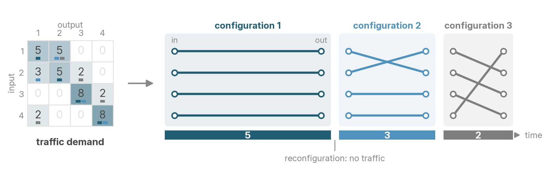
The article works with data of finite precision. The entries of the test matrices have three to seven decimal digits, and the method looks for exact decompositions whose weights have the same precision. If the entries are multiples of 1/s, for example s = 10⁴ for four decimal digits, the scaled matrix D = sA has integer entries and row and column sums equal to s, and a decomposition of D with integer weights c_l gives a BvN decomposition of A with λ_l = c_l/s. All computations can then be carried out in exact integer arithmetic, free of rounding errors. Figure 1 shows a small example, a 4 × 4 matrix scaled by s = 10, read as the traffic demand of a switch: its decomposition into three weighted permutation matrices is a schedule of three switch configurations.

Where it is used

The article names switch scheduling as the main application: each term of a decomposition is one switch configuration, and every reconfiguration costs time. Decompositions also arise in several other fields.

The Quantum Optimization Benchmarking Library (QOBLIB) includes the minimum Birkhoff decomposition problem among its test problems for quantum and classical methods, with 375 instances. These instances form the test set of the article.

What was known

The constructive proof of the theorem yields the Birkhoff algorithm: choose a permutation matrix whose ones lie on nonzero entries, subtract it with the largest weight that keeps the matrix nonnegative, and repeat. The usual choice is the bottleneck permutation, the one that admits the largest weight; such heuristics can miss the optimum. Variants such as Birkhoff+ choose each permutation matrix by a linear program, and Frank-Wolfe methods give good approximate decompositions but rarely exact ones. Exact methods go back to Minoux’s column generation approach, and mixed-integer programs solve small instances. The article reports no lower bound in the literature beyond the degree, the largest number of nonzero entries in any row or column: every term covers exactly one position in each row, so a row with five nonzero entries needs at least five terms.

One observation behind the method

The method rests on the line partition lemma. A line is a row or column. Each term of a decomposition covers exactly one position in each line, so every line partitions the weights into groups whose sums are its entries. In Figure 1, row 1 splits {5, 3, 2} into {5} and {3, 2}, and row 3 into {5, 3} and {2}. All lines share the weights; only the grouping differs. This holds for integer and real weights alike.

RCS is named after its three parts, Recover, Certify and Search, organized in two parallel chains. The solution chain (Recover and Search) builds decompositions, driving the best length k down. The bound chain (Certify) proves lower bounds, driving the bound L up. Every decomposition is verified in integer arithmetic before acceptance, and a run stops once k = L, which proves optimality.

Two classes of matrices need different tools. A matrix built from few permutation matrices, say n random ones, is sparse in the article’s sense: most entries are single weights, and values recur. One built from many, say n², is dense: every entry is a sum of many weights, no weight is visible, and the minimum length is far below the number of generating permutations. RCS is not told how a matrix was built; it treats a matrix as sparse if at least 45% of its nonzero entries have a value that occurs more than once.

Recover: reading the weights off a sparse matrix

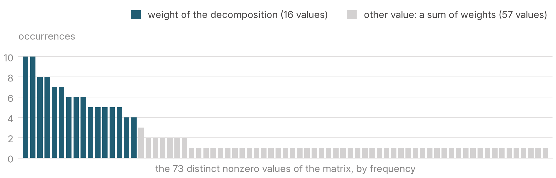
In a matrix built from n random permutations, a given permutation is the only one through its position in a given row with probability about 1/e, so its weight appears as an entry in about 37% of the rows. A sum of two weights appears only where two permutations meet, so the weights are the most frequent values (Figure 2). The frequency rule sorts the distinct values by frequency and takes the shortest prefix whose sum is exactly s, provided that the frequency drops there. If this fails, the values are scanned in increasing order, as in Jagabathula and Shah’s sparsest-fit algorithm.

The weights alone are not yet a decomposition: each must still be placed at the right positions. The article’s rule, fixing by unique subset sums, visits the open positions in increasing order of their entries. For each position, it lists those subsets of the weights not yet placed in its row and column whose sum equals the entry. If exactly one subset fits, the position is fixed to it. If none fits, the weights are wrong. If several fit, the position stays open, and a depth-first search settles the positions still open at the end. The article proves that, given correct weights, this rule never fixes a position incorrectly. Visiting small entries first keeps the subset lists short, because the smaller entries in the same row and column are usually fixed already.

Certify: proving that fewer terms are impossible

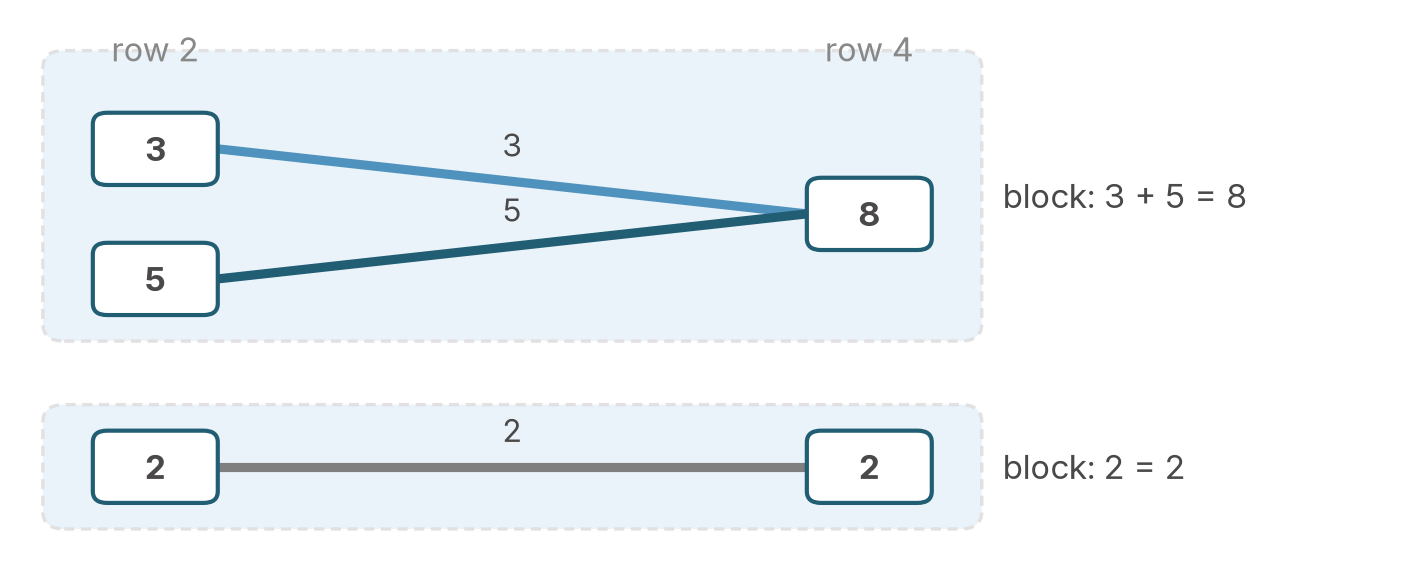
The bound chain raises the lower bound in three stages. The first is the degree. The second, the two-line bound, is the article’s central new bound. Take two lines with p and q nonzero entries. Every term covers one position in each of them and thus links these two positions. Positions that are linked, directly or indirectly, form groups in which the entries of the two lines have equal sums; any set of positions with this property is called a block. A group of r positions needs at least r − 1 links, so k ≥ p + q − γ*, where γ* is the largest number of blocks into which the entries of the two lines can be split (Figure 3). The bound depends only on the entries and, as the article proves, also holds for real weights. Equal values from the two lines can always form blocks of their own, so only the unmatched values require work. With at most 22 unmatched values, a dynamic program over subsets computes γ* exactly. With more, a linear program over small blocks gives a valid bound, its dual solution rounded and verified in integer arithmetic; with up to 44 unmatched values, a meet-in-the-middle enumeration still computes the exact value.

The third stage uses a Boolean satisfiability (SAT) solver. A SAT model decides whether D has a decomposition with k terms and integer weights; if it is unsatisfiable, at least k + 1 terms are needed. For small matrices, the question is split, cube-and-conquer style, into many independent cases, and many cases are eliminated by a lower bound on how many terms must cover each position. Unlike the degree and the two-line bound, a SAT certificate holds only for weights with the precision 1/s of the data, not for arbitrary real weights.

Search: building decompositions of dense matrices

In a dense matrix no weight is visible, so decompositions are built step by step. A zeroing step subtracts a permutation matrix with the largest weight that keeps all entries nonnegative, so at least one entry becomes zero. Among the bottleneck permutations, the zeroing rule picks one that zeroes as many entries as possible, and the Birkhoff algorithm with this rule gives the first decomposition of every run. A logarithmic tie-break rule breaks the remaining ties by removing as many binary digits from the remaining entries as possible; on dense matrices with n ≥ 32, one deterministic run of the Birkhoff algorithm with this rule gives decompositions 3 to 6% shorter than the zeroing rule alone.

The main search tool is a beam search over zeroing steps. It explores the tree of partial decompositions level by level, keeping only the most promising nodes per level, scored by the steps taken so far plus the steps the Birkhoff algorithm still needs. A node is pruned when its steps so far plus the degree of its residual (the matrix not yet decomposed) reach the length of the best known decomposition. For n ≤ 7, every permutation in the nonzero pattern is tried in every step, and the article proves that every decomposition with a so-called zeroing order is then a path in the tree. Further threads improve the best decomposition: a SAT re-optimization of the tail tries to replace its lightest terms with fewer ones, a large neighborhood search removes a group of related terms and re-decomposes their sum, and randomized restarts rerun the Birkhoff algorithm with random tie-breaking.

Results

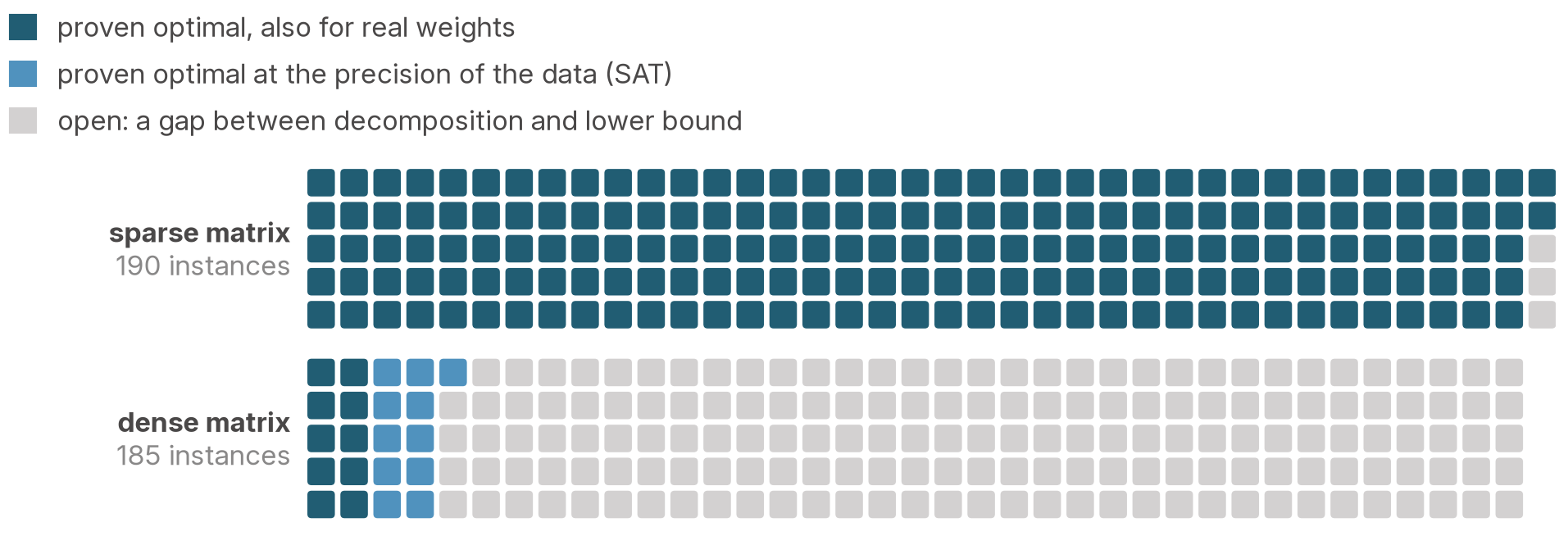
Of the 375 instances, 197 are proven optimal with proofs that hold for real weights, and 11 more by SAT certificates at the precision of the data (Figure 4).

Optimality. According to the article, the problem is solved in practice for sparse matrices: two lines of a sparse matrix share most of their values, and once equal values are paired off, the two-line bound proves optimality for 164 instances and the degree for 23. Only three sparse instances remain open, each with a gap of one term. The median time to the best decomposition is below 0.01 s, and the longest in any run is 0.07 s. For dense matrices, the two-line bound proves optimality for the ten instances with n = 3, again for real weights, and SAT certificates, valid only at the precision of the data, prove it for all instances with n = 4 and one with n = 5. Larger dense instances remain unproven.

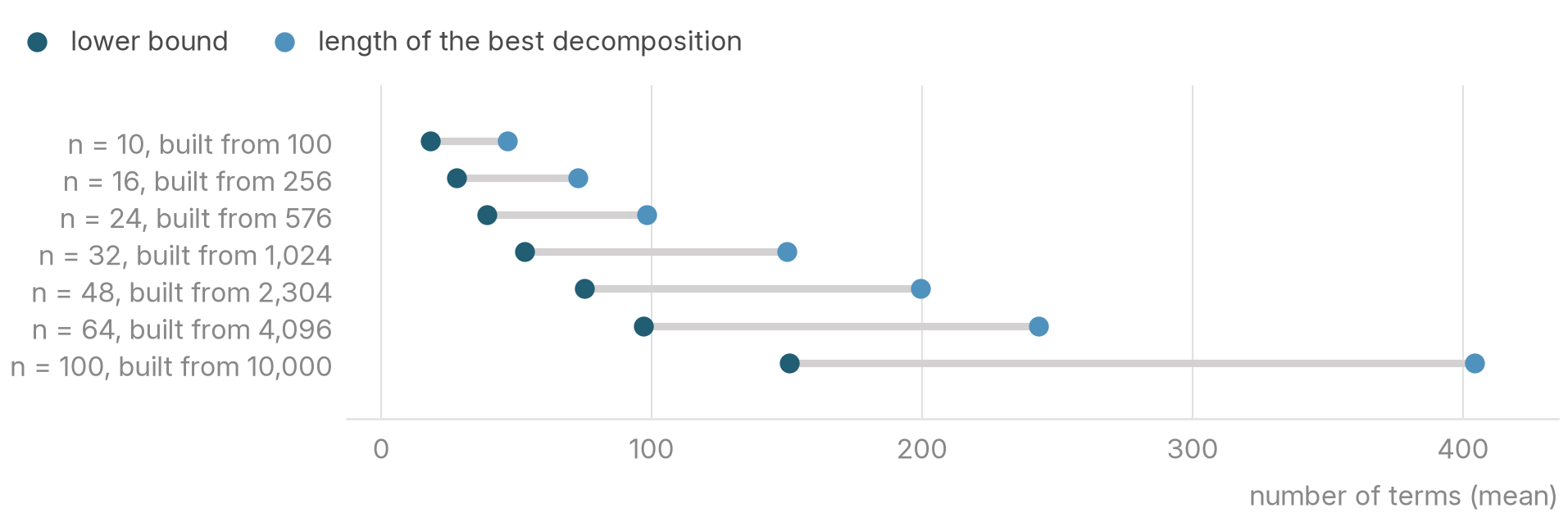
Dense matrices. Dense instances are built from n² permutation matrices, yet the decompositions found by RCS use only a small fraction of that many terms: for n ≥ 12, the mean length per size lies between 3.8n and 4.7n (Figure 5). The lower bounds stay near 1.6n for n ≥ 24, so for large dense matrices the decompositions are about 2.6 times as long as the bounds, and it is not known whether the bounds or the decompositions are farther from the optimum. The length divided by n jumps wherever the scale s grows tenfold (from n = 9 to 10, 24 to 32 and 64 to 100), so the precision of the data strongly affects it.

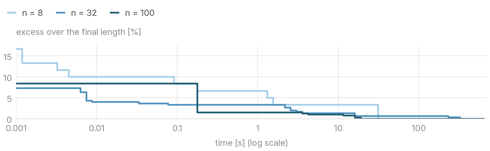
Running time. On dense matrices, the first decomposition is available in less than 0.2 s for every size, and most of the improvement happens within the first seconds (Figure 6). For 6 ≤ n ≤ 16, the median time to come within two terms of the final length is 0.4 s, and within one term 8.2 s; the last one or two terms take most of the running time. The beam search finds most of the best decompositions for dense instances with n ≤ 16, whereas for larger sizes the large neighborhood search, the SAT re-optimization of the tail and the randomized restarts make the final improvements.

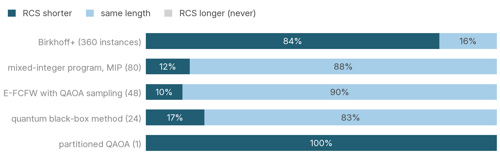
Comparison. Other groups have submitted results for these instances to the library. The article checks every submitted decomposition in integer arithmetic and counts it only if it reproduces the matrix exactly. Compared with the best of these, RCS is shorter on 278 instances, equal on 79 and never longer, and it gives the first exact decomposition for 18 instances (Figure 7). Birkhoff+ covers 360 instances and is fast, but its decompositions are on average 2.1 times as long. A mixed-integer program solved with Gurobi covers the 80 instances with n ≤ 6 and proves optimality for 66 of them, five more than RCS: on five dense instances with n = 5, RCS finds decompositions of the same length, but its lower bound stays one below. On the ten dense instances with n = 6, where the mixed-integer program stops at its time limit of two hours, the decompositions of RCS are shorter by one to three terms. The methods with quantum components (an extended Frank-Wolfe method whose candidate permutations are sampled by the quantum approximate optimization algorithm, QAOA, a quantum black-box optimization method and a partitioned variant of QAOA) give exact decompositions only for instances with n ≤ 8, apart from one with n = 16; RCS is never longer on them, and on that instance it needs 16 terms, not 66.

Limitations and open questions

The main open question is the gap for large dense matrices. The two-line bound alone cannot close this gap, because two lines of a dense matrix allow many blocks, so stronger bounds will need arguments that involve more lines. The SAT certificates hold only at the fixed precision of the data, and it remains open whether real weights allow shorter decompositions for matrices of this kind. The running time on large dense matrices is a practical problem, because the beam search spends most of it on greedy completions. Some ideas did not work: sampling vertices of the linear relaxation gave 16 to 17 terms on dense instances with n = 5 for which decompositions with 13 to 14 terms exist, and plain linear programming bounds were always weaker than the two-line bound.

Where to read more

The full scientific article, with all definitions, proofs, implementation details and per-instance results, is available on arXiv: arxiv.org/abs/2610.25837. The test instances are part of QOBLIB.